Ever wanted to implement a path tracer but didn’t know where to get started? Here I showcase my journey through one of the options: the Nori framework.

Nori is described as a “minimalist ray tracer written in C++” and was created for educational purposes by Wenzel Jakob and his team. Huge shoutout to them for making the course and the code available to the public.
I won’t go into detail of the techniques implemented in this course. More experienced people have created detailed resources for that. I’ll leave a link to the amazing Physically Based Rendering online book, which I visited frequently on my journey.

Implementing your own path tracer can be intimidating, especially if you start from scratch. Nori helps you to get started as it already comes with a lot of functionality and utility but leaves you with the implementation of core features such as a bottom level acceleration structure (BLAS), sampling techniques and different integrators.

The Course

So, how did I come to choose Nori? A while back in 2019 while attending a lecture about offline rendering at my university, we had assignments to implement path tracing techniques using Nori. Since then, the idea grew to follow through the original tasks of Nori in the back of my head. This summer I finally took the time and went through the course.

The concept of the course is really rewarding: You incrementally add features to your renderer until you have path tracing with multiple importance sampling. And you get working intermediates that show your progression. Seeing how my renderings improved helped my motivation big time. Also, you always get timings for your renderings, which gives you an idea of how expensive different techniques are.

The course is well-structured, however it requires you to do a fair amount of research yourself. While this was great training for me, as I had already heard about the techniques used in the course, it might be overwhelming if you are just getting started. You should be comfortable programming in C++ and background knowledge regarding Monte-Carlo integration will come in handy.

My Journey

I now present a series of renderings showing my progression through the course (I will skip some steps for brevity). I do this to give you a feeling of what to expect from the course and hopefully spark motivation to try it yourself.

The first setup tasks leave us with a visualization for normals. Here we get comfortable with the build chain and the framework itself.

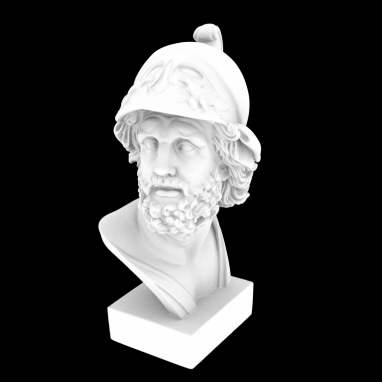
After the first setup tasks, we start to build our own acceleration structure, an octree. My implementation cut down the rendering time of the bunny scene from 9.2s to 535ms (plus 5ms to build the octree). This improvement in speed enables you to render the Ajax bust.

This scene rendered in roughly 14s (plus 1.7s to build the octree). I’d like to give you a timing without acceleration, but even after several minutes not a single 32×32 pixel block was rendered. Rendering complex scenes without acceleration structures is just not feasible.
After that we dive into Monte-Carlo integration, sampling and add an ambient occlusion integrator and direct diffuse lighting.

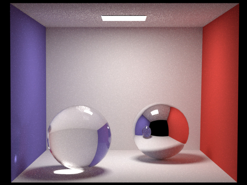
Now the ray tracing begins in Whitted-style, which adds reflection and refraction to our renderings.

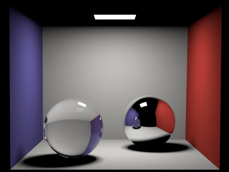
Indirect lighting is still missing, but we already have perfect reflection/refraction and even Fresnel on the glass sphere.

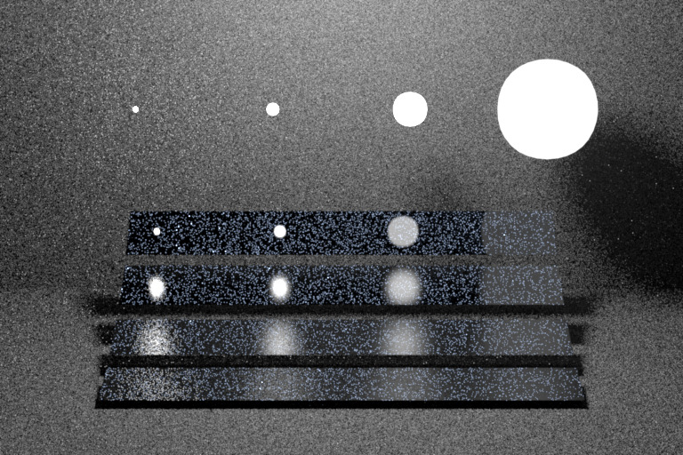
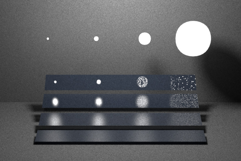
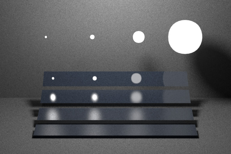
The next step is microfacet models. We dive into Bidirectional Reflectance Distribution Functions (BRDFs) and how to evaluate and sample them. Sampling different distributions and weighting them correctly was very intimidating to me as I first came across it. But it is crucial to all sampling based rendering techniques, and working with it took my initial fright of it. Seeing, how wrong weights affect your rendering or how a bad distribution creates noisy images improves your understanding, helps you see the need for good sampling practices and hopefully motivates you to dive into the math behind it.

Now it’s time for real path tracing. Our first implementation uses the surface material to generate light paths. We then add in next event estimation, which essentially means we sample the light sources in our scene. In the final step, we combine both techniques using multiple importance sampling, a core rendering technique developed by Veach.
We even get to imitate the iconic scene from the Veach paper.

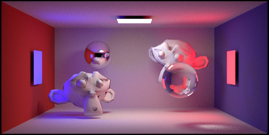
And finally, we can render our Cornell Box using path tracing!

Conclusion

After hearing a lot of theory on offline rendering, implementing core features of the process myself was a great experience. Really getting an understanding of a theory works best for me through practical application.

I hope this post provides guidance if you try to deepen your computer graphics programming skills, and maybe even sparks a bit of motivation to get into it. With that I leave you to it, hope you stay healthy in these trying times and wish you all the best!